Problem Description
We have a ciphertext that we have to decrypt in 48 hours. Luckily, one of our guys at the NSA was able to take a screenshot of the computer as it was performing the encryption, unfortunately it only captured part of the screen. Can you help us break the cipher?
- Difficulty: Hard
- Tags: Crypto
- author: 18lauey2
Attachments
TL;DR
Modified coppersmith method that converts the complex valued matrix into a real matrix through a canonical embedding and solve it like normal.
Introduction, audience, and pre-requisites
This writeup, like most of my writeups, is geared towards people with an elementary understanding of Math. Additionally, this writeup focuses on the logic behind the solution as opposed to just the solution.
The pre-requisites that would be nice to know before reading this are:
- The RSA encryption and decryption scheme Basic modular arithmetic Matrix algebra (vectors, linear combinations, and
-
matrices) An elementary understanding of complex numbers
Alright then. Sit tight and buckle up because we are in for a doozy!
Challenge Overview and Inspecting the Code
The challenge performs RSA with complex integers (Gaussian Integers: $\mathbb{Z}[i]$) as opposed to regular Integers $\mathbb{Z}$. A Complex integer is a complex number $a + bi$ such that $a, b \in \mathbb{Z}$.
Fortunately, the logic behind the algorithm, Complex-RSA (CRSA), remains fairly familiar with a few caveats:
- We say that a Gaussian integer $w$ is prime if its norm is prime.
- “What’s a norm?” In this case, consider a norm to be defined as $Re(w)^2 + Im(w)^2$. (This can be interpreted,
- geometrically, as the square of the point’s distance from the origin) Once we generate our primes
pandq, the rest of the process is the same as regular RSA. (I’m skipping over details for modular exponentiation because it’s not relevant to the challenge)
The second part of the challenge involves our LEAKed picture which features a terminal with output that reads the values
of N, ciphertext, and a some portion of p. Interestingly enough, we see about two-thirds of both the real and the
imaginary part of p with the rest covered by the beautiful hand-drawn raccoon
But we’re missing bits! Now what?
You’re right. There is still a bit of work to do if we would like to decrypt our message. Alright, let’s take a deep
breath and work step-by-step. What information do we need to retrieve the original plaintext m.
To decrypt a message we need d which is defined as e^-1 (mod (norm(p)-1)*(norm(q)-1)). To find d, we need p and
q which in turn require us to factor N = pq. To factorize N, we would need “recover” p from the information that
was leaked and divide N by p.
Oh boy. That’s a lot. All these steps are fairly straightforward with the exception of recovering p. So, our goal
is to recover this value.
After some painful counting and testing, There’s roughly about 155 digits for both the real and imaginary parts. we have about 85 and 87 of these digits respectively. (Okay, maybe it wasn’t two-thirds…)
Retrieving these missing bits seems hard. Let’s consider a simpler problem: What if this was regular RSA and we had about 60% of p. As it turns out, someone has solved this problem before.
A Copper sword crafted by the kingdom’s finest blackSmith
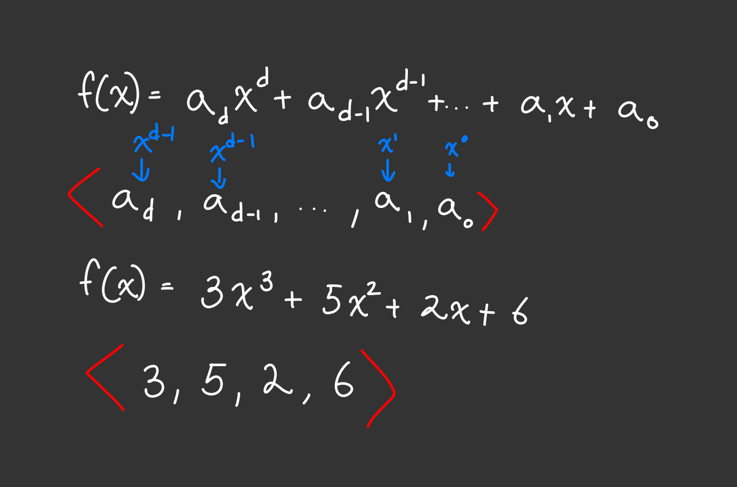
Enter the Coppersmith method. In a nutshell, the method finds small integer roots of polynomials modulo a given integer. To clarify, this means that if we have a polynomial of the form $F(x) = x^n + a_{n-1}x^{n-1} + … + a_1x + a_0$ where $a_i \in \mathbb{Z \text{ (mod N)}}$, and we know that there exists some integer $x_0$ such that $F(x_0) \equiv 0 \text{ (mod N)}$ and $|x_0|$ is less than $N^{\frac{1}{n}}$, we can find $x_0$.
You might be wondering, “cool fact. What does this have to do with us?” The answer is everything. Let me take you through this step-by-step.
- Recall that we have knowledge of
N, the fact thatN = p * q, and a fair chunk ofp(let’s say about 110 digits of 155 digits). - We can express
pas followsp = the_known_part + the_unknown_part. Mathematically, $p = a + r$ where a and r are the known and unknown parts of p respectively.- For example if
p = 382xx, we would express it as $p = 38200 + r$.
- For example if
- We also have that $r$ is less than $10^{45}$ since $r$ has 45 digits. Thus, we get an upper bound $R = 10^{45}$.
- Let’s create a polynomial $f(x)$ modulo $p$. We will define $f(x) = a + x$ where $a$ is a constant which represents
the known part of $p$.
- In the definition of the method above, $n = 1$ (aka the degree of the polynomial we must solve)
- Now, $f(r) = a + r = p \equiv 0 \text{ (mod p)}$. In other words, $r$ is our small ineger root $x_0$ from the definition above.
- Note, that $r$ is less than $R$ which is less than $p^{\frac{1}{1}} = p^1$ which is less than $N$.
- YAY! This is literally what the Coppersmith method needs to work.

The Coppersmith Attack is truly one of the attacks of all time
Now that we have the pieces, let’s apply the coppersmith method to find our $x_0$ ($r$). Firstly, it’s good to understand a bit of our motivation here. It is very difficult to find the roots of an integer polynomial over some modulo N. However, it is extremely trivial (relatively) to find the roots of the same polynomial over the integers. The method takes in our polynomial $f(x)$ performs a bit of magic and in combination with the Howgrave-Graham theorem it converts our polynomial modulo N to a simple polynomial with the same small roots over the integers (no modulo).
The Howgrave-Graham Theorem
Okay, so the (extremely abridged version of) Howgrave-Graham Theorem states that for a polynomial $g(x)$, if:
- $g(x_0) \equiv 0 \text{ (mod }b^k\text{)}$ for some $b, k$
- $abs(x_0) \le R$ Where R is the upper bound we discussed earlier
- The length of the coefficient vector of $g(R \cdot x)$ is small. (The coefficient vector refers to the vector containing the
coefficients of each term in our polynomial $[a_n, a_{n-1}, …, a_1, a_0]$.)
- Small is once again defined as being less than some bound based on $b, k$ and the degree of $g(x)$. However, it’s not relevant to us because we will fulfill it at the end. (Haha! this might be forshadowing)
then $g(x_0) = 0$ over the integers too. That is, $x_0$ is an integer root.
Great! let’s use this on $f(x)$. Well… we can’t use it just yet because the coefficients of the polynomial $f(R\cdot x)$ are huge. In particular, the constant term $a$ is the same number of digits of $p$. This fails the third condition in the Howgrave-Graham theorem which wants a small coefficient vector. Fortunately, there’s a way to fix this.
Reducing the Size of our Massive Polynomials
At first glance, it seems difficult to do reduce the size of our coefficients. However, all we need is a small cameo from our good old friend: linear combinations.
Suppose I had two polynomials $a(x)$ and $b(x)$ such that $a(x_0) \equiv b(x_0) \equiv 0 \text{ (mod m)}$ for some integers $m$ and $x_0$. Note that $a(x_0)$ doesn’t neccessarily equal $b(x_0)$. Now, we have that $a(x_0) + b(x_0) \equiv 0 \text{ (mod m)}$. Trivially, we also have that $l \cdot a(x_0) \equiv 0 \text{ mod(m)}$ for any integer $l$. Thus, for any integers $l$ and $k$, we get $l \cdot a(x_0) + k \cdot b(x_0) \equiv 0 \text{ mod(m)}$. So
In summary, we just showed that any integer linear combination of two polynomials preserves (or has the same) the root $x_0$ over our modulus $m$. So, this means that if we can find other polynomials which has the same root, x_0, as $f(Rx)$ (and $f(x)$) modulo $p$, then we can craft an integer linear combination between them to reduce the size of our coefficients. (Note: this is similar to the idea of row reductions in matrix algebra).
A Trick to Create Unlimited Polynomials
Our long chain of dominos continues as we search for polynomials with the same root $x_0$ as $f(x)$ over our modulus p. For convenience, I will call this set of polynomials $F$. The problem is we don’t know $p$, so we can’t make polynomials like $g(x) = px^2 + 4px + p^3$ which will always be 0 for all values of $x$. (They’re not particularly useful either). Let’s use some clever tricks instead.
- Firstly, we know $N$ which is a multiple of $p$ so $g(x) = N \equiv 0 \text{ (mod p)}$ for all $x$ including $x_0$. Let’s add it to $F$.
- Next, we have that $f(x_0) \equiv 0 \text{ (mod p)}$. We could square both sides and get: $[f(x_0)]^2 \equiv 0 \text{ (mod p)}. Nice! Let’s add $[f(Rx)]^2$ to $F$.
- Why stop there? We can just continue raising $f(Rx)$ to various ineger powers and have the same outcome as above. We can thus add all the powers of $f(Rx)$ to $F$.
Now, we have a long list of polynomials to choose from. An alternative to this method would be to simply multiply $f(Rx)$ by different powers of $x$. However, the downside to this method is that we would lose our constant term in the elements of $F$. The powers of $f(Rx)$ is much more elegant in the sense that due to the binomial theorem, we are bound to have constant terms.
The Magical Mysteries of the Lattice and LLL
We have a list of polynomials with the same root $x_0$ whose coefficients we seek to reduce through their integer linear combinations. It remains to be asked: “How do we determine the most efficient integer linear combinations”. It’s time to introduce Lattices and LLL.
Introducing our New Show: DeComplexify This!
Today, we will be learning what a Lattice and how LLL might help our little predicament. Recall that if we were working with the Real numbers, we could simply use a matrix to reduce the size of a basis and make it orthogonal using the gram schmidt method. However, we are working over the Integers where the same strategy cannot be used.
Introducing the Lattice. No, not the lattice from Organic Chemistry. An n x n (integer) lattice is essenitally just like a n x n matrix with two exceptions:
- All the elemwents in our lattice are integers
- The Span of our vectors refers to just the integer linear combinations. (Instead of real coefficients for matrices).
To clarify: We will exclusively be talking about integer lattices, hereby referred to as just lattices.
Like a matrix, we can put express our polynomial f(Rx) in the form of a row vector. In fact, you’ve already seen this before in the form of our coefficient vectors.
We can create a matrix using some of our polynomials in $F$ where each row is a polynomial and each column is represents the coefficients of a power of $x$. We can create a matrix using the polynomials $g(x) = N$, $f(Rx)$, $[f(Rx)]^2$.
Now that we have constructed our lattice, let me introduce the LLL algorithm (Lenstra-Lenstra-Lovász). I won’t be going over the nitty-gritty details of this algorithm and will instead treat this as a black box. This algorithm takes in a lattice basis (Basis has the same meaning as in matrix algebra) and outputs a lattice with a more orthogonal and smaller basis. You can read about it more in this wonderful tutorial. A fun exercise is justifying to yourself that our row vectors are linearly independent to each other.
Once we apply the LLL algorithm on this lattice, our rows, representing polynomials, will now have smaller coefficients. Since the length of our coefficient vector is smaller (by definition of LLL), we can apply Howgrave-Graham’s theorem in order to find $x_0$ by finding the roots of $h(x)$ over the integers. Note that the resulting row vectors will be of the form $h(Rx)$. We simply divide each coefficient by $R$ to retrieve $h(x)$.
We have succesfully found $r$ (our $x_0$) and we can reconstruct $p$ by $a + r$. Victory! We solved our simpler RSA problem. Now, to deal with something more complex. (literally)
The Complexities of Complex Numbers
The question now is: “Can we do the same for our complex integers?” The answer is mostly. While most of the theorems extends out to the Complex Integers, LLL only operates over the regular integers. To understand how we overcome this problem, let’s first go through our solution till our roadblock.
- Write down
Nand the known part ofpN = -117299665605343495500066013555546076891571528636736883265983243281045565874069282036132569271343532425435403925990694272204217691971976685920273893973797616802516331406709922157786766589075886459162920695874603236839806916925542657466542953678792969287219257233403203242858179791740250326198622797423733569670 + 617172569155876114160249979318183957086418478036314203819815011219450427773053947820677575617572314219592171759604357329173777288097332855501264419608220917546700717670558690359302077360008042395300149918398522094125315589513372914540059665197629643888216132356902179279651187843326175381385350379751159740993*I a = 1671911043329305519973004484847472037065973037107329742284724545409541682312778072234 * 10^70 + 193097758392744599866999513352336709963617764800771451559221624428090414152709219472155 * 10^68 * I - At the same time as finding
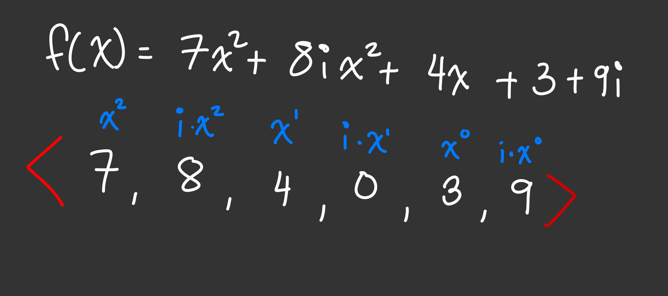
a, we can define our upper bound $R$ as $R_r$ and $R_i$ for the bound of the real and imaginary part ofr. Since the primes will always have about 155 digits (this could be verified with a bit of testing/bruteforcing other limits). - Our $f(x) = a + x$. Instead of this, we can choose to be more verbose and write it as $a + bi + x + i \cdot x$. Here, we treat $i$ similar to a variable and all the coefficients (like $a$ and $b$) are real integers.
- We do the same process as before to generate different powers of $f((R_r + R_i \cdot i)x)$ modulo p. (refer to the challenge code to see how you can take the modulo under a complex number)
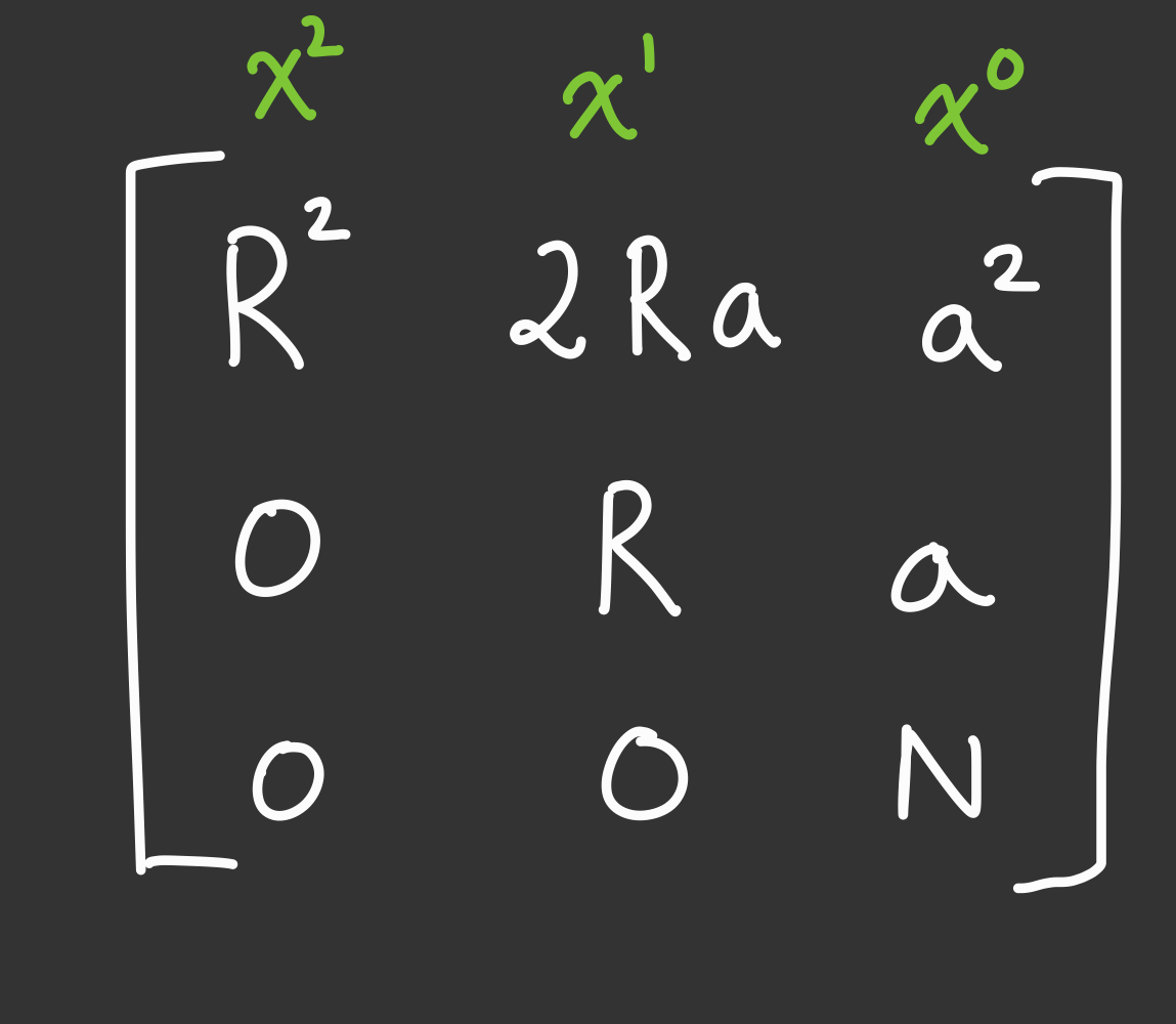
- Now, we hit our roadblock of representing our polynomials as row vectors of integers. Well, we could simply double
the columns (adding an imaginary part to each power of $x$). This looks like…
- one more note is that we can double our set from before by adding the imaginary multipe of $f$ such as $-i\cdot f(Rx)$
- Construct a matrix with a lot of these row vectors and perform LLL.
- The reason we need a lot of polynomials has to do with the Howgrave-Graham theorem which essenitally ends up equating to us requiring more rows to have a greater chance of finding our root.
- find the root of the reduced polynomial over the Complex Integers.
- Retrieve
rand thus find $p$ - Use $p$ to find $q$ and then find $d$ and use $d$ to decrypt our ciphertext given by:
e = 65537 ciphertext = 49273345737246996726590603353583355178086800698760969592130868354337851978351471620667942269644899697191123465795949428583500297970396171368191380368221413824213319974264518589870025675552877945771766939806196622646891697942424667182133501533291103995066016684839583945343041150542055544031158418413191646229 - 258624816670939796343917171898007336047104253546023541021805133600172647188279270782668737543819875707355397458629869509819636079018227591566061982865881273727207354775997401017597055968919568730868113094991808052722711447543117755613371129719806669399182197476597667418343491111520020195254569779326204447367 * I
Wow, we did it! oh no… It did not work :(
WHY DOESNT IT WORK!!
The short answer is that we need to modify our choice of polynomials because it still fails the conditions for the Howgrave-Graham Theorem. Recall that the Howgrave theorem limits us on our choices of $b$, $k$, and the degree of the polynomial. For the theorem, we need $f(x_0) \equiv 0 \text{ (mod }b^k\text{)}$. Previously, we just set $b^k = p$ and called it a day. However. However, through a long series of proofs that are very well highlighted on this blog, this can be very inefficient and makes it such that the maximum upper bound for $R$ ends up being very small. The maximum bound is usually defined by some relation $X \approx N^\frac{1}{c(d)}$ where $c(d)$ is a function that depends on the degree, $d$, of our polynomial. Understanding this, our goal would be to reduce the the growth of $c(d)$ as much as possible. We will be using two techniques to do this (from the same blog post).
The First Technique:
Rather than considering $b^k = p$, we could instead try $b = p$. This would ultimately help increase our upper bound (as described in the blog if you are curious). What changes? Well, unfortunately $f(x_0) \equiv 0 \text{ (mod }p^k\text{)}$ is no longer true. However, this might actually be useful.
I will leave this as an exercise to the curious readers, but it’s trivial to observe that if an integer $a$ divides $b$, then $a^k$ divides $b^k$. Also, if $a$ divides $c$, then $a^k$ divides $c^{i}b^{k - i}$ for some $i \in \mathbb{Z}$ that is less than $K$ and greater than zero. This implies that if we have two polynomials $a(x)$ and $b(x)$ such that $a(x_0) \equiv b(x_0) \equiv 0 \text{ (mod m)}$ for some integer $m$, then $[a(x_0)]^i[b(x_0)]^{k - i} \equiv 0 \text{ (mod }m^k\text{)}$.
So, let’s use the two polynomials we know are divisible by $p$ at $x_0$: $N$ and $f(Rx)$. (yes, N is a polynomial that equates to a constant.) Now, instead of using powers of $f(x)$, we can instead add polynomials of the form $[f(Rx)]^i[N]^{k - i}$ for each integer $i \in [0, k - 1]$ to our set $F$.
Note that for our complex integers, whenever I add a polynomial $g(x)$ to $F$, I’m also adding its imaginary multiple $-i\cdot g(x)$ to the set. This simply helps with the lattice reduction by giving the LLL algorithm more options to reduce our polynomials by.
Technique Numero Dos:
The second technique, which was discussed directly in the blog, involves multiplying $[f(Rx)]^k$ with various powers of $x$. Recall that $[f(x_0)]^k \equiv 0 \text{ (mod }p^k\text{)}$.So, we add polynomials of the form $[N]^i[f(Rx)]^k $ for each integer $i \in [0, k - 1]$ to our set $F$ (along with its imaginary multiples. Note that there’s nothing really stopping us from taking a different number of polynomials for the second technique, rather than $k - 1$ polynomials we can take $5$ or $4000$. Though I’m not sure what those bounds would be.
Back to business
Now that we have created a better lattice, we can finally solve our challenge. Nevermind! There’s a lot of sage-specific bugs that had to be squashed.
hours later, we can finally use our script to reverse the encryption and encoding to get our flag.
The solve script (finally)
from CRSA import GaussianRational, decrypt
from fractions import Fraction
from Crypto.Util.number import long_to_bytes
ciphertext = 49273345737246996726590603353583355178086800698760969592130868354337851978351471620667942269644899697191123465795949428583500297970396171368191380368221413824213319974264518589870025675552877945771766939806196622646891697942424667182133501533291103995066016684839583945343041150542055544031158418413191646229 - 258624816670939796343917171898007336047104253546023541021805133600172647188279270782668737543819875707355397458629869509819636079018227591566061982865881273727207354775997401017597055968919568730868113094991808052722711447543117755613371129719806669399182197476597667418343491111520020195254569779326204447367 * I
N = -117299665605343495500066013555546076891571528636736883265983243281045565874069282036132569271343532425435403925990694272204217691971976685920273893973797616802516331406709922157786766589075886459162920695874603236839806916925542657466542953678792969287219257233403203242858179791740250326198622797423733569670 + 617172569155876114160249979318183957086418478036314203819815011219450427773053947820677575617572314219592171759604357329173777288097332855501264419608220917546700717670558690359302077360008042395300149918398522094125315589513372914540059665197629643888216132356902179279651187843326175381385350379751159740993*I
a = 1671911043329305519973004484847472037065973037107329742284724545409541682312778072234 * 10^70 + 193097758392744599866999513352336709963617764800771451559221624428090414152709219472155 * 10^68 * I
# This function takes in our polynomial and returns two rows
# The first row is the coefficient vector, scaled by the uppper bounds, of the regular polynomial
# The second row is the coefficient vector, scaled by the upper bounds, of its imaginary multiple
def get_coefficients(f, R_r, R_i):
regular = []
imag_multiple = []
coeffs = f.list()
for i, c in enumerate(coeffs):
regular.extend([c.real() * R_r^i, c.imag() * R_i^i])
for i, c in enumerate(coeffs):
imag_multiple.extend([-1 * c.imag() * R_r^i, c.real() * R_i^i])
return [regular, imag_multiple]
# since our row vectors have different lengths, we need to pad them with zeros
# Note that the solve script reverses the columns. The leftmost column is the constant while
# the rightmost column is the coefficient of the highest degree of x
def rpad(lst, length):
result = []
for l in lst:
result.append(l + [0 for i in range(length - len(l))])
return result
def coppersmith(f, R_r, R_i, N, k):
# This was the maximum number of columns/entries a row vector has.
max_cols = 4 * k
# polynomial row vectors
polynomial_rows = []
x = f.parent().gen(0) # apparently helps sage do its thing
# Add polynomials from our first technique
for i in range(k):
poly_rows = get_coefficients(f^i * N^(k-i), R_r, R_i)
poly_rows = rpad(poly_rows, max_cols)
polynomial_rows.extend(poly_rows)
# Add polynomials from our second technique
for i in range(k):
poly_rows = get_coefficients(f^k * x^i, R_r, R_i)
poly_rows = rpad(poly_rows, max_cols)
polynomial_rows.extend(poly_rows)
# We perform LLL on our lattice
M = matrix(polynomial_rows)
B = M.LLL()
# v is the first polynomial from our reduced lattice
v = B[0]
# This section was lifted from the official solve, but just cleans up our polynomial
Q = 0
for (s, i) in enumerate(list(range(0, len(v), 2))):
z = v[i] / (R_r^s) + v[i+1] / (R_i^s) * I
Q += z * x^s
return Q
R.<x> = PolynomialRing(I.parent(), "x") # sage once again doing its thing
f = x + a # our beloved polynomial
# 10 seemed to be the sweet spot
Q = coppersmith(f, 10^70, 10^68, N, k=10)
# r = x_0 = Q.roots()[0][0]
p = a + Q.roots()[0][0]
# Now we cast the values we calculated to GaussianRationals and find q
p = GaussianRational(Fraction(int(p.real())), Fraction(int(p.imag())))
N = GaussianRational(Fraction(int(N.real())), Fraction(int(N.imag())))
ciphertext = GaussianRational(Fraction(int(ciphertext.real())), Fraction(int(ciphertext.imag())))
q = N / p
# calculate the value of d from p and q
p_norm = int(p.real*p.real + p.imag*p.imag)
q_norm = int(q.real*q.real + q.imag*q.imag)
tot = (p_norm - 1) * (q_norm - 1)
e = 65537
d = pow(e, -1, tot)
# decrypt our ciphertext
m = decrypt(ciphertext, (N, d))
# decode the message
print(long_to_bytes(int(m.real)) + long_to_bytes(int((m.imag))))
Flage
SDCTF{lll_15_k1ng_45879340409310} Indeed it is king.
Final Thoughts
This was a really hard challenge. I spent over 30 hours straight running in circles with various techniques like complex LLL and Algebraic LLL. However, I did not solve this challenge at the end of the CTF. In fact, this challenge went unsolved by anyone. After discussing with the author, I realized that one of my earlier ideas of converting the complex integers to a real matrix to do LLL was actually the intended solution. However, I didn’t quite understand how to complete the solve path which was doing a canonical embedding. An embedding is similar to what we did with using different columns for the real and imaginary part of the powers of $x$ and using the imaginary multiples.
I’m glad I was able to solve it regardless because it’s better late than never. More importantly, I hope that this guide can give you some understanding behind the complexities of the coppersmith method often needed for RSA challenges. In this vein, I have another section with resources I found useful for this challenge.
Finally, shoutout to 18lauey2 for making such a cool challenge.
Resources to help my dumb dumb brain
- A bunch of lectures from Tanja Lange on Coppersmith and RSA as part of 2MMMC10 at Eindhoven University of Technology https://www.youtube.com/@tanjalangecryptology783/videos
- The blog written by Cousin Wu Ka Lok from
blackb6ahttps://www.klwu.co/maths-in-crypto/lattice-2/#second-idea - The paper the challenge was inspired by Ideal forms of Coppersmith’s theorem and Guruswami-Sudan list decoding
- A wonderful paper that summarizes the various attacks on RSA. Recovering cryptographic keys from partial information, by example
That’s all folks.